SwissOrthology Guide
Welcome
Welcome to the SwissOrthology Flowchart. Here, you can interactively find information to help guide you to choose between different SwissOrthology tools. For some applications, either OMA or OrthoDB is better suited. For others, both orthology resources are fine. In the flowchart, you can interactively decide which resource to use based on one of the following criteria:
Click on one of the above to begin exploring how SwissOrthology can work for you.
Species in OMA and OrthoDB
Both OMA and OrthoDB predict orthologs for a diversity of animal, plant, fungal, and bacterial genomes.
OMA predicts orthologs over many species, including animal, fungal, plant, archaea, bacteria. The latest OMA release (Aug 2020) covers 2326 species. OMA also infers orthologs across kingdoms. A full list of species and their update dates is available on the release information page.
OrthoDB’s latest release predicts orthologs among 7275 species and 6488 viruses: 448 metazoan, 117 plant, 549 fungal, 148 protist, 5609 bacterial, 404 archaeal genomes, and 6488 viruses, picking up the best sequenced and annotated representatives for each species or operational taxonomic unit. The latest species list can be found here.
Additional information:
- OrthoDB additionally infers orthologs among viral genomes.
- Don’t find your species? You can suggest it for the next OMA release.
- OrthoDB offers the possibility to analyse your genome of interest online by mapping to existing orthologous groups.
Species in OrthoDB
In addition to the 7275 eukaryotic, bacteria, and archaea species, OrthoDB v10 covers 6488 viruses.
Using your own species in analysis
Both OMA and OrthoDB allow for using your own sequenced genomes as input data.
The OMA pipeline can run on custom genomic/transcriptomic data using the OMA standalone software, and it is even possible to combine precomputed data with custom data by exporting parts of the OMA database, which saves time on the all-against-all step.
The OrthoDB software is also freely available from https://www.orthodb.org/software.
Additionally, in OrthoDB users can upload and analyze online their genome of interest. As many genomes are newly sequenced and analysis is needed for the first publication, OrthoDB has the possibility for users to create a registered account. After uploading the data, the analysis is performed automatically. The registered user can then see the OrthoDB interface with the new data and benefit from annotations of related orthologous groups in OrthoDB and other dababases.
Identify all orthologs of a gene in a given set of organisms
- I want pairwise orthologs between my favorite gene and specific genomes of interest
- I want orthologous groups (clusters of genes from multiple genomes)
Additional information:
- Do you want to include paralogs?
- Do you want to include homoeologs?
Pairwise orthologs
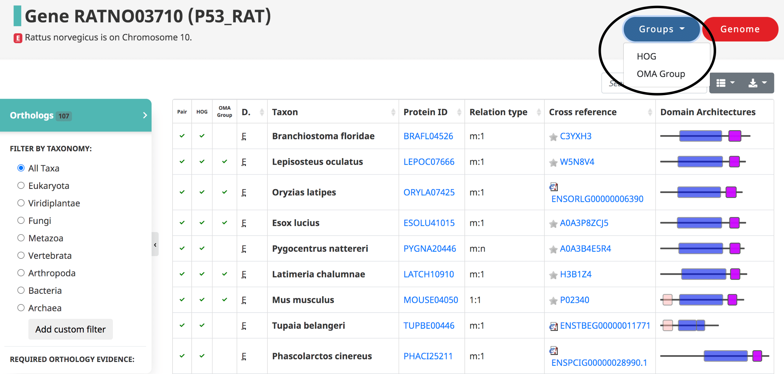
The OMA Browser reports different subtypes of orthologous and paralogous relationships.
Evolutionary relationships are often described as pairwise relationships. Pairwise orthologs in OMA are those which are inferred at the base of the OMA algorithm. They are formed by looking for the evolutionarily closest protein sequences between two genomes within a confidence interval.
Users can find a list of all ortholog pairs for a given gene of interest by searching for their gene on the omabrowser. See the OMA Manual: Orthologs of a Given Gene on how to find pairwise orthologs, HOG-induced orthologs, and OMA-induced orthologs.
Alternatively, users can download a list of all predicted ortholog pairs between genomes of interest. The result is returned as a tab-separated text file.
https://omabrowser.org/oma/uses/Additional information:
OMA reports the relationship cardinality of the pairwise orthologs, which reflects the level of co-orthology, or the degree of duplications which one or both of the orthologs has undergone. One-to-one (1:1) pairwise orthology means that both genes in the pair have only one ortholog in the other species. A one-to-many relationship (1:m) means that the gene of interest has more than one ortholog in the other species. This implies that the gene was duplicated in an ancestor of the other species, but after the speciation event. A many-to-many (m:m) relationship means both orthologs underwent lineage-specific duplications.
OrthoDB reports the phyletic profile for each ortholog group. It is a summary of the ortholog presence (from universal to species-specific) and copy-numbers (single/multi-copy counts). For example, orthologous Group 125711at40674 at Mammalia level (functionally annotated as Cellular tumor antigen p53) contains 116 genes in 109 species (out of 111). It is single copy in 102 species, and multi-copy in 7 species.
Orthologous groups
Both OMA and OrthoDB report groups of orthologous genes.
OrthoDB was the first database to introduce hierarchical orthologous groups. The concept of orthologous groups is inherently hierarchical, as each phylogenetic clade or subclade of species has a distinct common ancestor. The ortholog delineation procedure is applied at each major radiation of the species taxonomy to produce more finely resolved groups of closely related species and to allow users to select the most relevant level.
OMA also reports Hierarchical Orthologous Groups or HOGs. HOGs are sets of genes that are defined with respect to particular taxonomic ranges of interest. They group genes that have descended from a single common ancestral genes in that taxonomic range. Currently, HOGs can be accessed by searching for a specific HOG id or by a member gene of the group. To get to a HOG through one of its member gene pages, click on the “Groups” tab in the upper right-hand corner.
For more detailed information, see Access the OMA Data: Group-centric pages. Additionally, all the HOGs from the current release can be downloaded in OrthoXML format and parsed and analysed with pyham.
Another type of orthologous group that OMA reports are called OMA Groups. OMA groups contain sets of genes which are all orthologous to one another within group. This implies that there is at most one entry from each species in a group. OMA Groups can equally be accessed by searching for an OMA Group id or through the Groups tab on any gene-centric page of the browser.
Additional information:
Differences between different types of orthologs in OMA
OMA reports three “types” of orthologs: pairwise-induced orthologs,Hierarchical Orthologous Groups (HOGs)-induced orthologs, and OMA Group-induced orthologs. These are three different methods, so they might not report identical orthologs. However, HOG and OMA Group orthologs are based on pairwise orthologs so they should be similar. For more information, see: Differents types of homologs in OMA.
| Pairwise orthologs | Hierarchical Orthologous Groups (HOGs) | OMA Groups | |
|---|---|---|---|
| Algorithm | Built by mutually-closest protein sequences within a confidence interval | Built by merging groups of pairwise orthologs at different taxonomic levels using a guide tree | Built by searching for cliques of pairwise orthologs (i.e. all genes that are pairwise orthologs to all others in the group) |
| Genomes included | Compares 2 genomes at a time | Compares all genomes at a time | Compares all genomes at a time |
| Types of homologs | Strictly orthologs, but can be 1:m or n:m. | Groups of orthologs and in-paralogs for a specific speciation event of reference. | Strictly orthologs, at most 1 per species reported, although there may be more not reported. |
Additional information:
- Introduction to HOGs YouTube video
- Altenhoff et al. 2015
- Zahn-Zabal et al. 2020
Paralogs
Both OMA and OrthoDB report paralogs.
Paralogs are those genes which started diverging due to a duplication.
In OMA, paralogs are derived from the HOGs, inferred from duplication events. Thus, any pair of genes in the same species and the same HOG are in-paralogs with respect to the defined taxonomic level of the HOG.
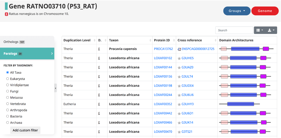
Paralogs can be accessed in the OMA browser from the gene-centric pages by clicking on the Paralogs tab from the side-menu. They are defined in OMA by the taxonomic level at which the duplication occurred. The resulting table displays the duplication level, domain of life, taxon (species in which the paralog is found), protein ids, cross references, and domain architectures.
OrthoDB reports in-paralogs with respect to a given taxonomic level. Users can see online or download paralogs in orthologous groups; the paralogs are genes from the same species in the same orthologous group.
How do in-paralogs relate to 1:1, 1:many and many:many orthology relations?
Homoeologs
OMA reports homoeologs for allopolyploid species in the database.
Homoeologs are pairs of genes that originated by speciation and were brought back together in the same genome by allopolyploidization. Homoeologs can be thought of as orthologs between subgenomes.
OMA reports homoeologs for 4 species: Triticum aestivum (bread wheat), Gossypium hirsutum (upland cotton), Brassica napus (rapeseed), and Xenopus laevis (African clawed frog).
Additional information:
- Glover et al. 2016. Homoeologs: What Are They and How Do We Infer Them? Trends in Plant Science.
Identify orthologous marker genes to infer a species tree
Both OMA and OrthoDB provide orthologous marker genes.
Orthologous marker genes (also known as phylogenetic marker genes) are sets of genes which are all orthologous to one another within the group. These marker genes should be 1:1, implying that there is at most one entry from each species in a group, and thus these marker genes are especially useful when creating a phylogenetics tree-- the gene tree will should match the species tree.
OMA identifies cliques of orthologous pairs (“OMA groups”), which are especially useful as marker genes for phylogenetic reconstruction and tend to be very specific. Since many users are only interested in a small subset of genomes, there is a function to retrieve, for a given subset of species, the most complete OMA groups. This functionality, entitled ‘Export marker genes’, is accessible under the ‘Download’ menu. Users can optionally choose a minimum proportion of species present in each group (‘occupancy’), and a maximum number of groups to export. From the choice of species and parameters, the OMA server identifies the most complete groups and produces a compressed archive file containing one fasta file per marker gene (i.e. per OMA group).
For a full description of the Export Marker Genes tool, see Catalog of Tools: Phylogenetic Marker Gene Export.
OrthoDB identifies single copy Orthologous Groups (OGs): groups with 1:1 representatives in all (or >90%, >80%) of species, as well as universal orthologous groups, meaning groups with members present in all (or >90%, >80%) of species at any selected taxonomic level. Using such filters, users can choose the numbers of OGs they want to build a species tree at the level of interest.
Build a gene tree
It is possible to obtain gene families, or groups of orthologous genes, from both OMA and OrthoDB, which are necessary to build a gene tree.
In OMA, you can obtain the HOGs, which are groups orthologs and paralogs which descended from a common ancestral gene at any given taxonomic level. To streamline the process of building a gene tree, you can:
- Search for your favorite gene on the OMA browser, then go to the HOG table view.
- Or, search for your HOG of interest directly using the HOG id or one of its member genes.
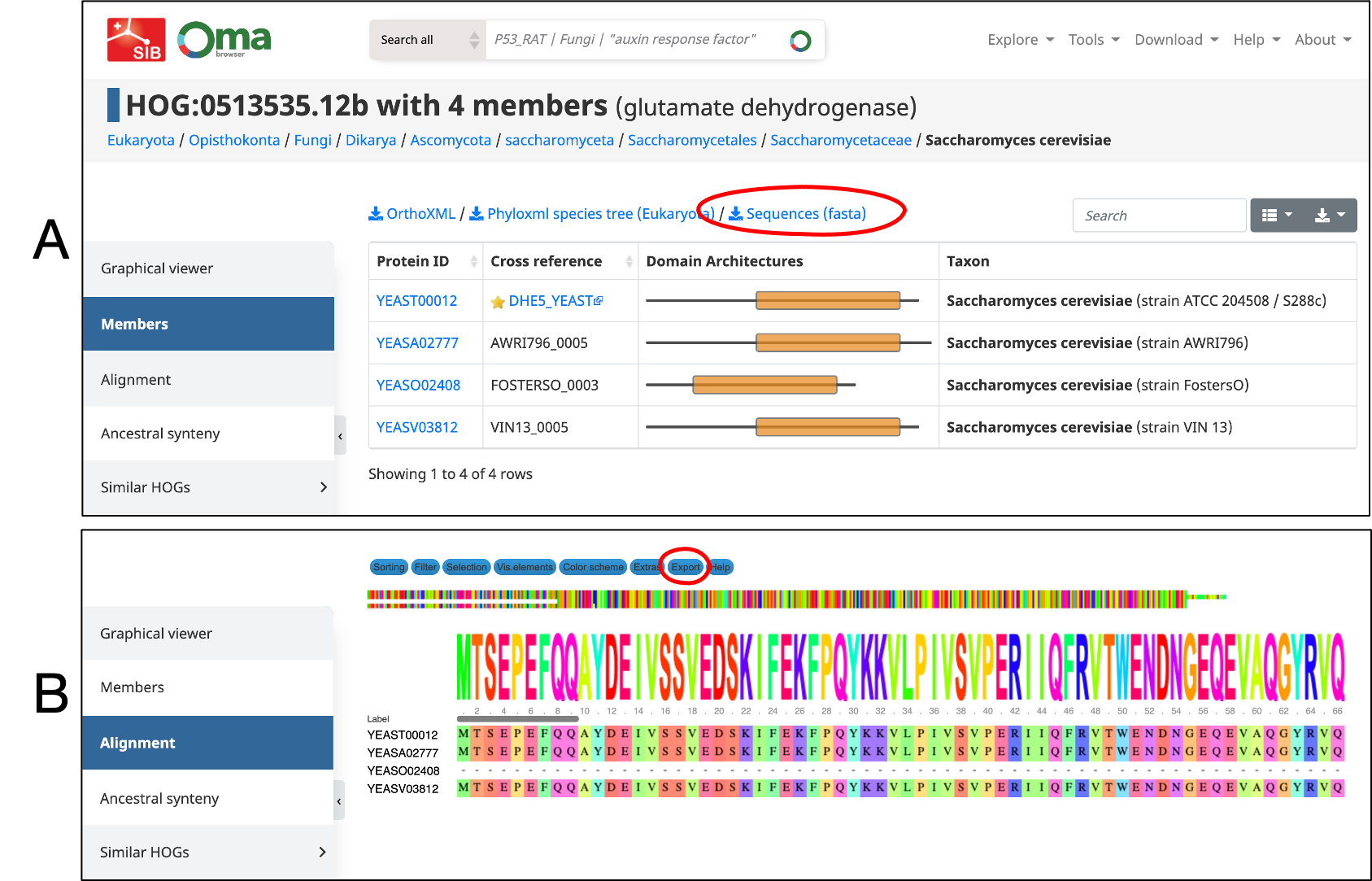
- Download the fasta sequences directly from the HOG table.
- Or, export the Mafft multiple sequence alignment (accessible from the side menu).
- Use the MSA in an external tree-building software.
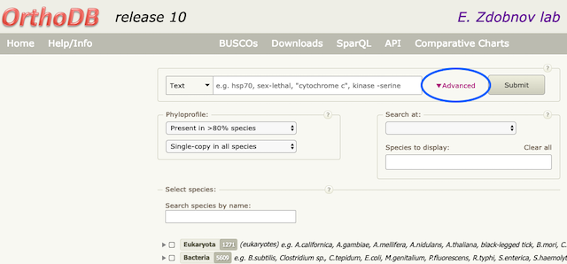
OrthoDB provides an “Advanced” search with a PhyloProfile option. There, one can select single copy groups for tree building. “PhyloProfile” allows the user to filter single-copy orthologous groups and their presence in most species (100%, 90% or 80%); this can be done at a selected taxonomic level, as well as coupled with specific annotations (i.e. certain functions). Afterwards, sequences for selected groups can be downloaded in an unaligned Fasta format and usedto build a MSA and a tree.
Additional information:
Trace the evolutionary history of a gene family
OMA lets you trace the evolutionary history of a gene family in terms of gene duplications and losses.
The evolutionary history of gene families can be complex due to duplications and losses. As provided by several orthology databases, hierarchical orthologous groups (HOGs) are sets of genes that are inferred to have descended from a common ancestral gene within a species clade. By keeping track of HOG composition along the species tree, it is possible to infer the emergence, duplications and losses of genes within a gene family of interest.
The OMA browser allows for viewing HOGs with an interactive widget called iham to visualize and explore gene family history encoded in HOGs. Additionally, one can query the HOGs for evolutionary events programmatically using the python library called pyham.
See the guide: How to Get the Evolutionary History of Your Favorite Gene in OMA to find out how to get to and use iham. You can also learn more about iham by watching the YouTube tutorial.
OrthoDB for each orthologous group offers the following set of evolutionary descriptors: Phyletic Profile, Duplicability, Evolutionary Rate and Gene Architecture.
- Phyletic profile that reflects gene universality, i.e. proportion of species with at least one ortholog in a particular ortholog group,
- Duplicability that reflects the proportion of multi-copy versus single-copy orthologs in an ortholog group,
- Evolutionary rate that reflects the relative conservation or divergence of protein sequence,
- Gene architecture that reflects the observed variations of the protein lengths and exon counts of the member orthologs.
Additional information
- Train et al. 2018. iHam and pyHam: visualizing and processing hierarchical orthologous groups. Bioinformatics.
- Blog post: pyHam: a python package to visualize and process hierarchical orthologous groups (HOGs)
Find the synteny between two genomes
Synteny is the conservation of gene order and/or overall chromosomal location. Synteny can be viewed on a global or local level, where global synteny looks at the overall chromosomal conservation, and local synteny looks in a smaller neighborhood for conservation of gene homology and order.
Export orthologs between two genomes to use in an external synteny software
Both OMA and OrthoDB let you export orthologs for external synteny packages.
Many synteny programs exist for computation and visualization of syntenic regions between two genomes, such as i-ADHoRe, MCScanX, circos, among others. Generally the input for these programs is a text file of pairwise orthologous relations or orthologous groups.
With OMA you can download pairs of orthologs between two genomes or HOGs. With OrthoDB you can download HOGs.
Visualize global synteny between two chromosomes
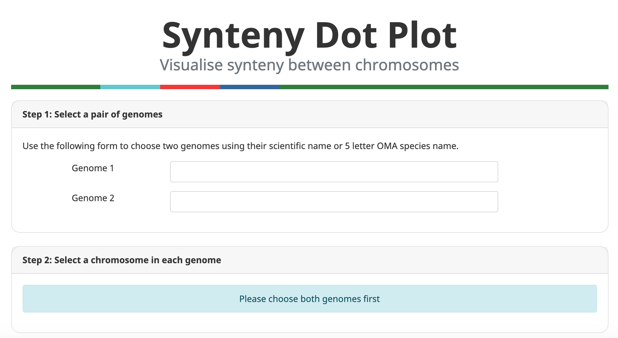
OMA lets you visualize the global synteny between two chromosomes of different or the same genomes.
These are the steps to use the OMA Synteny Dot Plot:
- Select the two genomes you want to compare. If comparing two different genomes, by default the dots on the plot represent orthologs, with paralogs being optional. If you compare the same genome, OMA will display
paralogs. If the same genome is an allopolyploid (wheat, brassica napus, or cotton), you will display
homoeologs and/or
paralogs
between subgenomes.
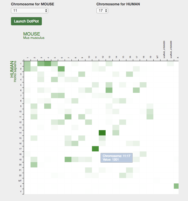
- After choosing the genomes, a heatmap will appear below showing where the frequency
of
orthologous relations are between the two genomes. This is to get an overall idea
which
chromosomes are conserved, because the higher number the orthologs per chromosome
pair
indicates
a higher synteny.
- The Synteny Dotplot is then displayed, where each dot is a pairwise orthologous
relation
between
the two chromosomes. There are several options here, with buttons in the upper right
hand corner
of the diagram.
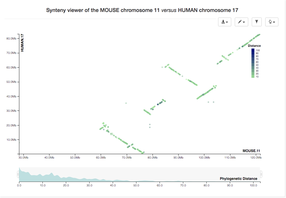
A wide range of operations can then be applied to the selected chromosome pair:
- You can export the file as an image
- You can filter which dots to display based on the type of homologous relationship (1:1,1:m, m:n, close paralogs, homoeologs).
- You can filter the dots by Evolutionary/Phylogenetic distance. This is computed as part of the normal OMA algorithm and based on sequence similarity. Click on the icon to display the histogram the bottom, from which you can move the bounding filters on the left and right.
- You can zoom in and zoom out with the mouse.
- You can select a region to display more information about the homologs (dots) in that region.
Local synteny
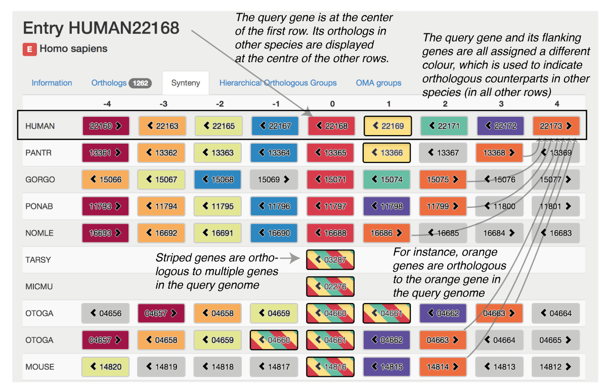
OMA allows for visualization of local synteny.
The synteny view provides an overview of the genomic context of a particular entry and its orthologs in other species. This enables to see conservation or divergence of syntenic regions across species. As synteny is computed with respect to a reference entry, one can first search for a protein sequence of interest and click on the “Local Synteny” tab. Equally, one can directly access the Local Synteny Viewer from the home page -> Explore.
Domain annotations of proteins
Both OMA and OrthoDB report domain annotations for the proteins in the databases.
OMA integrates domain annotations from Gene3D for individual protein entries. For each protein, the sequence of annotated domains is depicted using the conventional ‘colored-boxes-on-a-line’ representation, which we include in most protein lists. This makes it possible to easily check whether the domain architecture of a protein is conserved among orthologs, or to identify entries which are likely to be truncated or otherwise problematic. CATH domains (28) are depicted in colors specific to their first and second level classification.
OrthoDB provides InterPro attributes associated with individual member proteins. Additionally, at the group level, domain information is summerized.
Domain-based links between orthologous groups
Both OMA and OrthoDB assign domains to orthologous groups and allow for retrieving related groups based on domains.
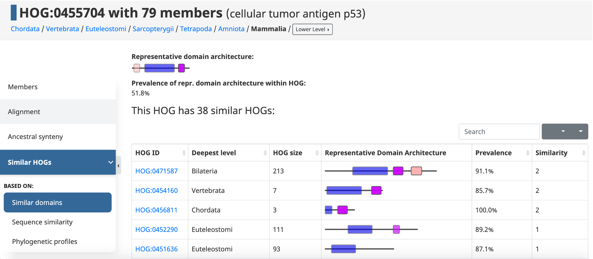
In OMA, domains can be used to establish links between HOGs. Given an initial HOG, a user can retrieve a table of the most similar HOGs based on conserved domain architecture. This domain architecture view allows users to estimate how specific or widespread the domains that make up a protein family are, and allows them to make hypotheses about the origin of a protein family.
OrthoDB has a section, Sibling groups, that reflects the sequence non-uniqueness by the fraction of InterPro domains shared with other groups of orthologs. Related groups are ranked by sequence overlap. For each sibling group list of InterPro domains is displayed, users see domain-domain rearrangements at a glance.
Gene Ontology
An important application of orthology is the ability to transfer gene function annotations from the few well-studied model organisms to the large number of poorly studied genomes. Gene Ontology (GO) is a way of consistently organizing annotated functions of genes.
Obtain GO annotations for proteins
Both OMA and OrthoDB report GO annotations for proteins in their databases.
One key motivation for orthology inference is to computationally predict the roles that genes play in living organisms—e.g. Cellular Component, Molecular Function and Biological Process of the Gene Ontology. Gene Ontology (GO) annotations from the UniProt-GOA database have been linked to all sequences in OMA, as well as inferred annotations based on orthology relationships: within the orthologous groups, OMA propagates GO annotations across different species. Amongst the available annotations, most are computationally inferred; OMA’s own predictions constitute about 20% of the available annotations. In OrthoDB currently, about 51% of clusters have GO annotation.
Additional information:
- Gene Ontology
- 2015 NAR OMA paper explaining the function prediction algorithm in OMA
Obtain GO annotations for orthologous groups
OrthoDB provides GO annotations for orthologous groups.
In OrthoDB, Gene Ontology and InterPro attributes associated with individual member proteins provide a general description for the Orthologous Group as a whole. These are summed over the member proteins to indicate the most frequently occurring attributes associated with the Orthologous Group.
Make your own GO annotations
OMA now provides a feature to annotate custom protein sequences through a fast approximate search with all the sequences in OMA. The user can upload a fasta formatted file and will receive the GO annotations (GAF 2.1 format) based on the closest sequence in OMA. These results can directly be further analyzed using other tools, e.g. to perform a gene enrichment analysis. This functionality is accessible under the Compute menu in the OMA browser.
I want to choose a resource based on output data
OMA and OrthoDB both provide access to their orthology predictions in various formats:
- OrthoXML format
- OMA provides for OrthoXML files for each individual Hierarchical Orthologous Groups (HOGs), all HOGs at once as well as for all OMA Groups.
- Fasta files
- OMA: Individual and all protein sequences and cDNA sequences, protein sequences for pairwise orthologs, HOGs per taxonomic level, and OMA Group
- OrthoDB: All proteins from your selected species from all orthologous groups that match your search
- REST API (primarily json)
- Text format:
- OMA: OMA groups, HOGs, pairwise orthologs, protein annotations, identifier mappings, species information: (Taxon IDs, scientific names, genome sources), group descriptions
- OrthoDB: all proteins from your selected species from all orthologous groups that match your search, xrefs associated with Ortho DB gene
- Other
- OMA: Json, XML, SQL, MS-Excel, CSV (HOGs), SeqXML format for protein sequences, HDF5 pytable (full OMA Browser database dump), OMA Groups/Sequences in COGs format, and PhyloXML for the species phylogeny of HOGs